Neural Network from First Principles
The purpose of this article is to understand the neural network from the first principles so that it feels more like a sequence of explicit, interpretable operations instead of a blackbox. We will build the intuition for every component including forward pass, shapes, matrix multiplication, loss function and backpropagation. I will reduce the blackbox into a composite linear algebra and calculus.
Neural network can be seen as a web of interconnected neurons, which mimics human brain. It takes inputs adds weights and biases with activation function to introduce non-linearity. During training the model learns from the loss function using a method called backpropagation and adjust the weights accordingly.
Forward Pass
Forward pass is the process in which the data flows from the input to the output layer. Forward pass is nothing but a composite function to make a prediction. It takes the input X apply weight and add bias. At each neuron we take a dot product of input array and weights metrics and add a bias term and then apply the activation function.
Thus at each node we calculate:
$$Z_1 = W_1 \cdot X + b$$
At each layer we have weights (edges), biases and activation function.
$$Z^{[n]} = \sigma(W^{[n]} @ X^{[n - 1]} + b^{[n]})$$
where:
- W = weight matrics
- X = input the the layer
- b = the bias
- \(\sigma\) = sigmoid activation function
Shape
the inner shape must me equal for dot product
- \(w: (m,n) @ x: (n,b) + b(m,1) = z1\)
- for batch
- \(w: (m,n) @ x: (n,batch) + b(m,batch) = z1\)
Activation Functions
We need activation function to introduce non-linearity.
Forward Pass
# forward pass using 2 loops
input = [1,2]
weights = [[1,2], # weights connecting to neuron 1
[2,3], # weights connecting to neuron 2
[3,4]] # weights connecting to neuron 3

biases = [1,2,3]

# forward pass z
def forward_pass(input, weights, biases):
	z = []

	for i in range(len(weights)):    #loop over the rows in weights
		neuron = 0
		for j in range(len(input)):                 # loop over elements
			neuron += input[j] * weights[i][j]
			neuron += biases[i]
		z.append(neuron)
		return z
Simple 3 layer Neural Net Forward Pass
## we learn tha the shape must match i.e. the inner shape must be same for dot product calculation
## note: @ is dot product and use broadcasting and vectorization
### example a: (m, n) @ b: (n, b) a's column = b's row. -> (n,b)
### in Weights the first dim m represents the number of neurons and n represents the number of inputs x coming from previous layer
### the activation function is carried to next layer
### z1 = W @ x + b -> a1 = relu(z1) -> z2 = W2 @ a1 + b -> a2 = relu(z2).....
import numpy as np

def relu(z):
	return np.maximum(0, z)

np.random.seed(42)

# layer 1
w1 = np.random.randn(6,4) * 0.1 # 6 neurons * 4 inputs
b1 = np.random.randn(6)

# layer 2
w2 = np.random.randn(4,6) * 0.1
b2 = np.random.randn(4)

# layer 3
w3 = np.random.randn(2,4) * 0.1
b3 = np.random.randn(2)

def forward_pass_nn(x):
	# l1
	z1 = w1 @ x + b1
	a1 = relu(z1)

	# l2
	z2 = w2 @ a1 + b2
	a2 = relu(z2)

	# l3
	z3 = w3 @ a2 + b3
	a3 = relu(z3)
	return a3

x = np.array([1.0,2.0,3.0,1.0])
forward_pass_nn(x)
Backpropagation
Backpropagation is used to train the neural networks by computing gradient of a loss function wrt to the weights of the network. It iterates backward thorough the network one layer at a time using chain rule. The idea is to minimize the loss function using gradient descent optimization.
The first step is to calculate the error. A loss function tells how bad the predictions are compared to the real or ground truth. A loss value is calculated for the whole network which tell us how bad our network is performing. The most simplest error function is MAE or Mean Absolute Error. It calculates the average of the absolute difference.
Lets, say
- \(\hat{y}\) is predicted values and
- \(y\) is ground truth
$$MAE = 1/n \sum_{i=1}^{n} (\hat{y} - y)$$
However, we are interested in the MSE or Mean Squared Error as it it continuous differentiable unlike MAE which is not differentiable at zero and have constant slope which is an issue for gradient decent. Mean Squared Error also penalize big outliers as the difference is squared, since it is continuous it converges faster.
$$MSE = 1/n \sum_{i=1}^{n} (\hat{y} - y)^2$$
Gradient Descent
Gradient decent is an iterative optimization algorithm that find the minimum of a loss function by repeatedly taking step towards the opposite direction of the gradient. Imagine you're traveling downhill without knowing the deepest valley. In simple terms gradient is a vector that contains all the partial derivatives of a multivariable function.
For gradient decent to work the loss function must be continuous and smooth (differentiable).
So the idea is to minimize the loss function to get the best combination of weights and biases, we assume that a global minimum exist for the data. For a scalar quantity with one variable its just the derivative of the function.
Calculating the Gradient of a Function
Given function:
$$ f(x) = x² - 4x + 5 $$
The goal is to find the \(x*\) such that the \(f(x*)\) is minimum. Thus we take the derivative of the function
$$f'(x) = 2x - 4$$
The second derivative of the function is positive and hence the function is concave and the minima exist.
$$f''(x) = 2$$
Now, instead of using the analytical approach we use an iterative approach
$$x_{n+1} = x_n - α * f'(x_n)$$
where:
- \(α\) = a learning rate or step size
\(f'(x_n) > 0\) then we move left (as function is increasing)
\(f'(x_n) < 0\) then we move right (as function is decreasing)
The learning rate hence is an important hyper-parameter which is required to be tune. If its sets too high, it will overshoot the minimum and oscillates and if its too low then the model will converge too slow. Its usually a small positive number which scales the gradient to update the model weights and controls the learning rate (how fast and slow).
Since in real world we model multivariate problems, we move to multivariate calculus. Consider function \(f(x)\), where \(x = [x_1, x_2, ..... x_n]^T \in \mathbb{R}^n\)
$$ ∇f(x) = [∂f/∂x₁, ∂f/∂x₂, ..., ∂f/∂xₙ]ᵀ $$
The gradient vector is pointing towards the steepest ascent and hence to minimize the loss we take the \(-∇f(x)\)
Now since we have multiple parameters (weights and biases) to tune we can represent them in matrix form using \(\theta\) parameter thus,
$$ \theta = [w_1(:), b_1, w_2(:), b_2.....w_n(:), b_n]^T $$
therefore, \(\theta\) is nothing but a column vector of weights and biases
Iterative gradient decent of the neural network will be
$$θ_{n+1} = θ_n - α * ∇L(θ_n)......(1)$$
However we have thousands of weights and biases and to calculate each partial derivative to find the gradient will be very slow. Therefore, we use the chain rule. Chain rule helps us to compute the gradient in one backward pass, this is the backpropagation of errors.
Backpropagation using Chain Rule
The idea is since, the neural net is nothing but a nested/composite function, we can use chain rule. So we are essentially asking how individual weight \(W_{i,j}\) contribute to the Loss \(L\)
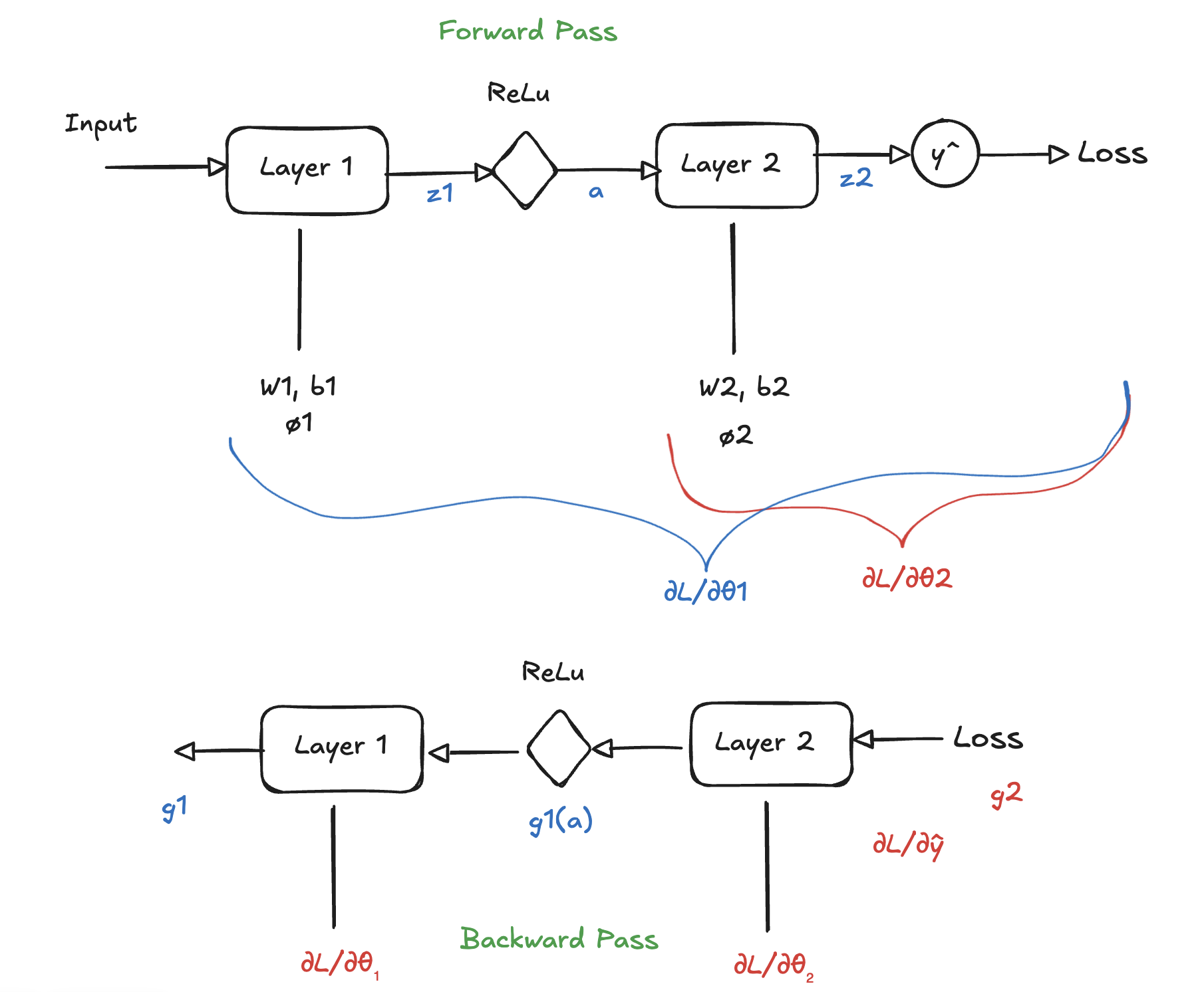
We need to calculate the gradient at each layer:
Gradient at layer 2 is given by:
$$\frac{\partial L}{\partial \theta_2} = \frac{\partial L}{\partial \hat{y}} \cdot \frac{\partial \hat{y}}{\partial z^2} \cdot \frac{\partial z^2}{\partial \theta_2}$$
For \(\theta_1\):
$$\frac{\partial L}{\partial \theta_1} = \frac{\partial L}{\partial \hat{y}} \cdot \frac{\partial \hat{y}}{\partial z_2} \cdot \frac{\partial z_2}{\partial a_1} \cdot \frac{\partial a_1}{\partial z_1} \cdot \frac{\partial z_1}{\partial \theta_1}$$
The term \(\frac{\partial a_1}{\partial z_1}\) is activation lets say ReLu which is 1 if \(Z_1 > 0\)
Notice that the term \(\frac{\partial L}{\partial \hat{y}} \cdot \frac{\partial \hat{y}}{\partial z_2}\) is repeated again in both the equation, and hence we can compute them once and store it.
therefore the equation becomes:
$$g_1 = g_2 \cdot \frac{\partial a_1}{\partial z_2} \cdot \frac{\partial z_1}{\partial a_1}$$
where \(g_2 = \frac{\partial L}{\partial \hat{y}} \cdot \frac{\partial \hat{y}}{\partial z_2}\)
Or recursively we can use:
$$\delta^{l-1} = \left( (W^l)^T \delta^l \right) \odot \sigma'(z^{l-1})$$
which means that each layer uses the gradient from the layer after it. This is the reason we go backwards. Its saves unnecessary gradient computation. Hence, neural net can be seen as a big composite function. To minimize loss we need gradients for all the parameters. Computing each gradient independently is inefficient and using the backpropagation algorithm we can compute gradients and update the new weights using equation (1).
The elegance of backpropagation is it transforms the high dimensional optimization problem into a simple bookkeeping, where each neuron just know its own local derivative, by multiplying these rate of changes the network communicate the global error.
Complete Neural Network
import numpy as np

def relu(z):
    return np.maximum(0.0, z)

def relu_deriv(z):
    # d/dz ReLU(z)
    return (z > 0.0).astype(z.dtype)

# Complete Multi layer perceptron regressor
class MLPRegressor:
    """
    forward: caches z and a at each layer
    backward: computes grads dW, db using chain rule
    step: SGD update
    """

    def __init__(self, layer_sizes, seed=42, weight_scale=0.1):
        assert len(layer_sizes) >= 2
        self.layer_sizes = layer_sizes
        self.L = len(layer_sizes) - 1  # number of weight layers

        rng = np.random.default_rng(seed)
        self.W = {}
        self.b = {}
        for l in range(1, self.L + 1):
            in_dim = layer_sizes[l - 1]
            out_dim = layer_sizes[l]
            self.W[l] = rng.standard_normal((out_dim, in_dim)) * weight_scale
            self.b[l] = np.zeros((out_dim, 1))

        self.cache = {}
        self.grads = {}

    def forward(self, X):
        """
        X: shape (d_in, batch)
        Returns Yhat: shape (d_out, batch)
        """
        self.cache = {"A0": X}
        A = X

        for l in range(1, self.L + 1):
            Z = self.W[l] @ A + self.b[l]  # (out_dim, batch)
            self.cache[f"Z{l}"] = Z

            if l < self.L:
                A = relu(Z)
            else:
                A = Z  # linear output for regression

            self.cache[f"A{l}"] = A

        return A

    def loss_mse(self, Yhat, Y):
        """
        Yhat, Y: shape (d_out, batch)
        """
        diff = Yhat - Y
        return np.mean(diff * diff)

    def backward(self, Y):
        """
        Compute gradients for all layers.
        Y: shape (d_out, batch)
        """
        self.grads = {}
        Yhat = self.cache[f"A{self.L}"]
        batch = Y.shape[1]

        # MSE: L = mean((Yhat - Y)^2)
        # dL/dYhat = (2/(d_out*batch)) * (Yhat - Y)
        d_out = Y.shape[0]
        dA = (2.0 / (d_out * batch)) * (Yhat - Y)  # (d_out, batch)

        for l in range(self.L, 0, -1):
            A_prev = self.cache[f"A{l-1}"]          # (in_dim, batch)
            Z = self.cache[f"Z{l}"]                 # (out_dim, batch)

            if l < self.L:
                dZ = dA * relu_deriv(Z)             # (out_dim, batch)
            else:
                dZ = dA                              # linear output => dZ = dA

            # dW = dZ @ A_prev^T / batch
            dW = (dZ @ A_prev.T) / batch            # (out_dim, in_dim)
            db = np.mean(dZ, axis=1, keepdims=True) # (out_dim, 1)

            self.grads[f"dW{l}"] = dW
            self.grads[f"db{l}"] = db

            if l > 1:
	            # propagate to previous activation: dA_prev = W^T @ dZ
                dA = self.W[l].T @ dZ               # (in_dim, batch)

        return self.grads

    def step(self, lr=1e-2):
        """
        SGD parameter update
        """
        for l in range(1, self.L + 1):
            self.W[l] -= lr * self.grads[f"dW{l}"]
            self.b[l] -= lr * self.grads[f"db{l}"]

    def train_step(self, X, Y, lr=1e-2):
        """
        forward -> loss -> backward -> update (full iteration)
        """
        Yhat = self.forward(X)
        loss = self.loss_mse(Yhat, Y)
        self.backward(Y)
        self.step(lr)
        return loss
On Training
To train a model we batch our data into small chunks to avoid memory constraints, faster training and convergence. Batching also prevents overfitting as training in small batches introduce noise and avoid sharp local minima, which can happen in large datasets. The weights are updated after every iteration. We train our model multiple times which is called Epoch. Epoch and Batch is simple hyper-parameters of the model which governs the over and under-fitting of the model.
References